One of the big things I wanted to achieve during this HDR project is to have a decent tone and gamut map filter, something Krita never had all these years, in spite of us having unbounded floating point editing as well as color management via LCMS that works with this unbounded floating point.
The unbounded floating point allows us to have values that might be (0.0, 0.5, 1.0) in linear rec2020, and then when converted to linear sRGB this becomes (-0.37, 0.56, 1.0). Now, the range of each channel here is [0 1], so if we try to represent that as an inbounds sRGB colour (which we need to do if we want to save for web), the default behaviour is to clip the out-of-bounds values, so we get (0.0, 0.56, 1.0). This changes the proportion between the blue and the red and green channels, meaning the hue and saturation will shift. In some cases, it can cause colours to gradually shift to values like (0.0, 1.0, 1.0). This is, for example, why your phone camera won’t shoot that lovely orange sunset just right: The colors are too colourful and get pushed towards yellow due clipping. So to combat this, you do gamut mapping: you shift the colour in bounds by a certain algorithm before or after doing the conversion.
Gamut Mapping
The most common gamut mapping algorithm is chroma-reduction. This assumes that the target space and the source space have their greys at the same location (taking into account white point adaptation). Then, the colors are converted to a third space, a opponent color space that also has its greys in the same location.
Opponent color spaces are spaces where the luminosity are separate from the chromacity and hue, and the chromacity and hue themselves are expressed as a red-green and a yellow-blue contrast, following the opponent theory of human color vision. A typical example of an opponent color space is LAB, but there’s many others, like YCbCr, ICtCp and OkLAB. These opponent colorspaces can then be translated to a Hue, Chroma and Luminosity space by treating the red-green and blue-yellow contrasts as Carthesian coordinates, and converting those to polar coordinates, giving us hue as the angle, and chroma as the length.
Then, for chroma reduction, you do a binary search to find the edge of the gamut, with each iteration, increasing the chroma or decreasing it, until the difference between the desaturated color, and the clipped version of the color is below a significant difference. That significant difference is called the minimum delta E, E being the name given to color difference by itself.
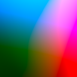
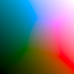
Shown above: a slice of LAB chromacity plane, with a black-to-white gradient diagonally. The first image is plain clipping to sRGB, while the second uses chroma reduction gamut mapping. In the first image, the chroma of the colors bottomleft and topright are so bright that when clipping they end up way with the wrong luminosity than they should have in reality. By doing chroma reduction, we pull these colours so far back in that their luminosity is preserved.
Krita implements CSS-4’s chroma reduction method, and offers it with 3 different opponent spaces: LAB, ICtCp and OkLAB.
This is because the delta E calculation for LAB is a little off, in particular, LAB is known to give weird results with the blue, with bright blues looking a little purple in LAB. ICtCp and OkLAB are much more modern and are particularly designed to have much better handling of the blue hues, which is visible in the gamut mapping:

ICtCp and OkLAB also had the advantage of being possible to implement in an ad-hoc manner starting from XYZ, so I didn’t need to integrate them directly into our color management system yet.
Besides binary search, there’s the cusp method. Here, you figure out the luminosity and maximum chroma of a given hue (the cusp), and use that to approximate the gamut boundary. There’s two ways to calculate the cusp:
The first is to use 6 polynomials, but that method only works with OkLAB as the opponent space and target RGB spaces that are matrix shapers. This in turns had to do with the simplicity of OkLAB as a colour space compared to other opponent spaces.
The second is to create a look up table of cusps per hue. Here, you take the known cusps in the target colour space and convert them to the opponent space to get their chroma and luminosity. This works for both CMYK and RGB spaces, as we know the likely cusps for those: Red, Yellow, Green, Cyan, Blue and Magenta and the interpolations between those. It also works with LAB, ICtCp and OkLAB equally. I went with this second method for now, but the first method is going to be more precise, and is worth investigating.
With the cusp for a given hue, you can then draw a triangle, going from black, to the cusp, to the reference white of the target space (important to keep in mind when combined with ICtCp-pq!), and back to black. The maximum chroma for a given lightness can then be derived by calculating the intersection between the current chroma and luminosity, and the zero chroma (grey) version of said luminosity.
Both the CSS4 gamut edge seeker algorithm and Ottoson’s algorithm use a curved top (cusp to reference white) section for the triangle here, but I am skeptical that this is strictly necessary. The colour only needs to be pushed into gamut enough so that once you clip it doesn’t cause massive hue and luminosity changes.
The interesting thing about the cusp method is that with the location of the cusp, you can decide to not just intersect with the grey of a given luminosity, but instead draw the line slightly towards the luminosity of the cusp. Bjorn Ottoson has a blogpost with experiments demonstrating this, and while not right now implemented in Krita, I would like to give it a go in the future as it can give more chromatic results.
There’s other methods. Scaling (“chroma compression”) methods, for example, generate a histogram of chromacity and lightness at a given hue-angle in the input image, and then the same for the target gamut. The resulting algorithm then doesn’t need to do any binary search, but can just scale the chromacity of the input by taking the maximum source chroma and scaling it by the maximum target chroma. This is also not yet implemented in Krita, but it might be interesting for CMYK output. Technically this is what ICC’s perceptual and saturation intents are all about, but those suffer from being too generic: a desaturated image that is fully in-gamut for the target space will get treated with the same lookup table as a fully saturated image, leading to odd results. A image-specific filter might give much better results.
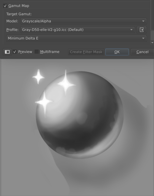
Finally, when the target space is greyscale, we don’t bother with either method and just set the saturation to 0.
Tone Mapping
Tone mapping is a subset of gamut mapping, where we only try to get the full range of tones (luminosity) into a target range. This is used to prepare HDR images for SDR output.
This is typically done by applying a so-called “filmic” curve. The name “filmic” derives from these curves mimicking real world chemical film’s tone properties, which when mapped onto a graph somewhat resembles a flattened “S”. The top part of this S-shape is referred to as the “shoulder” and the bottom part the “knee”, or, because it is quite tiny compared to the “shoulder”, the “toe”.

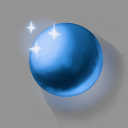
In the following section I’ll be using a picture of a blue orb on a grey background with some sparkles. I drew the original image on an HDR display, and it’s brightest highlights are around 8.0 (8 times higher than the reference white). Because most people don’t own a HDR display, I’m not going to try and share the image. Instead, I’m sharing the above image with two different exposures: The first is 0 exposure, it just clips all the colors. The second is with -2 exposure, showing how the highlights are supposed to look, but now the shadows are too dark. What we are looking for in the following images is that the sparkles are distinct from the highlight on the orb. That the blues look nice and don’t hue shift too much and that the shadows are not too light or too dark.
When looking for curves to implement, I wanted to have curves that were user configurable. So the first curve I implemented was the extended Reinhard curve. This is a pretty well known solution and the curve allows selecting the maximum white that gets mapped to 1.0. While it has a nice shoulder, it doesn’t have a knee or toe of any kind, which means it loses the contrast that is present in the HDR image.
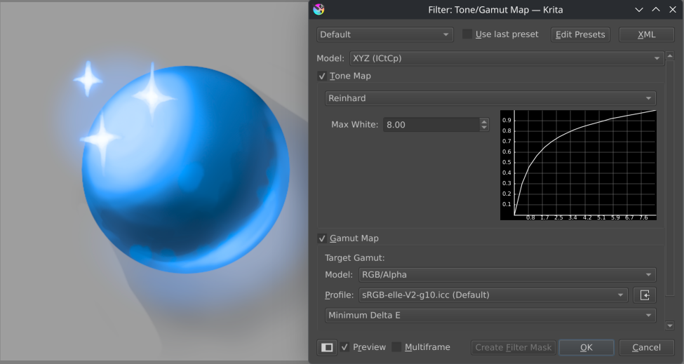
I then briefly looked at the Hermetic Filmic Curve as described by bt 2390-8, which has both a shoulder and knee. However, that one is applied in the PQ transfer instead of linear light, and the PQ transfer requires decisions about the brightness of the reference white, so I wasn’t sure how to do that one properly.
Then, I came across John Hable’s Piecewise Filmic Curve: A very configurable curve which has various parameters for editing the shoulder and toe. It takes a bit to configure, but as you can see, once configured, it preserves the contrast quite well:
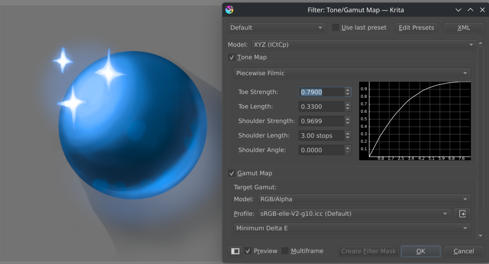
I implemented both curves on top of LAB, and xyY. This means that they’re applied to the luminance channel only.
Frequently, you will see the discussion on whether to apply the tone mapping to individual channels, or to apply it to a Luminance channel only. The base argument for using individual channels is that it’ll give chroma reduction as the colour will get lighter. The argument for applying it on a luminance channel is that it is more radiometrically correct. Though, it is correct that the bright colors now become more chromatic.
This is because to get the luminance channel, the colors need to be converted to a opponent space (typically, xyY, for easy conversion). But, when dealing with ‘hdr’ colours, like (3.0, 2.0, 0), it is not just the brightness that is high, but also the chroma. When tone mapping in an opponent space, the chroma is untouched. This leads to overly chromatic colours near the bright highlights, and these chromatic colours differ per opponent color model:
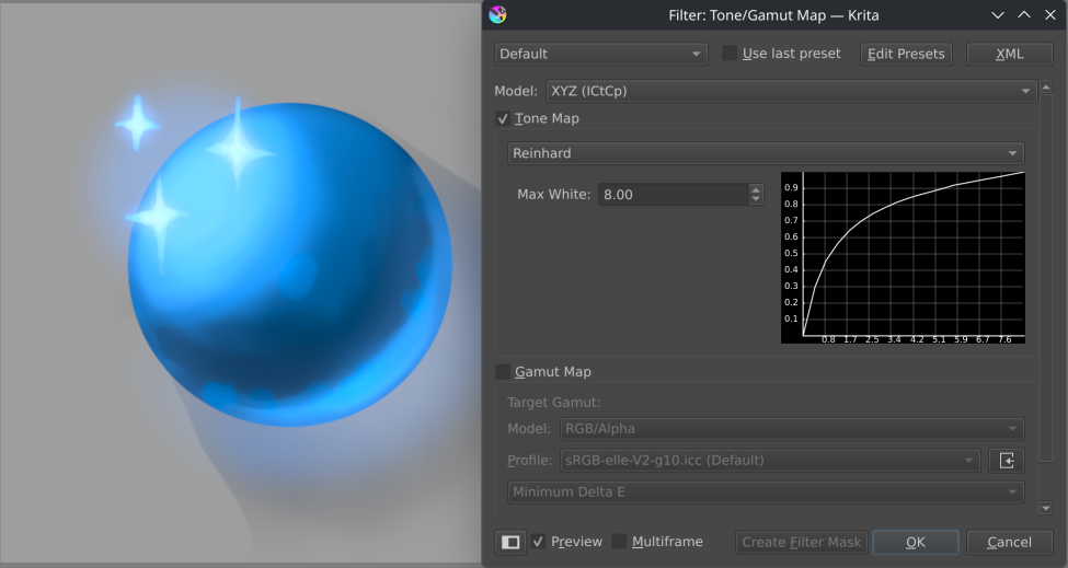
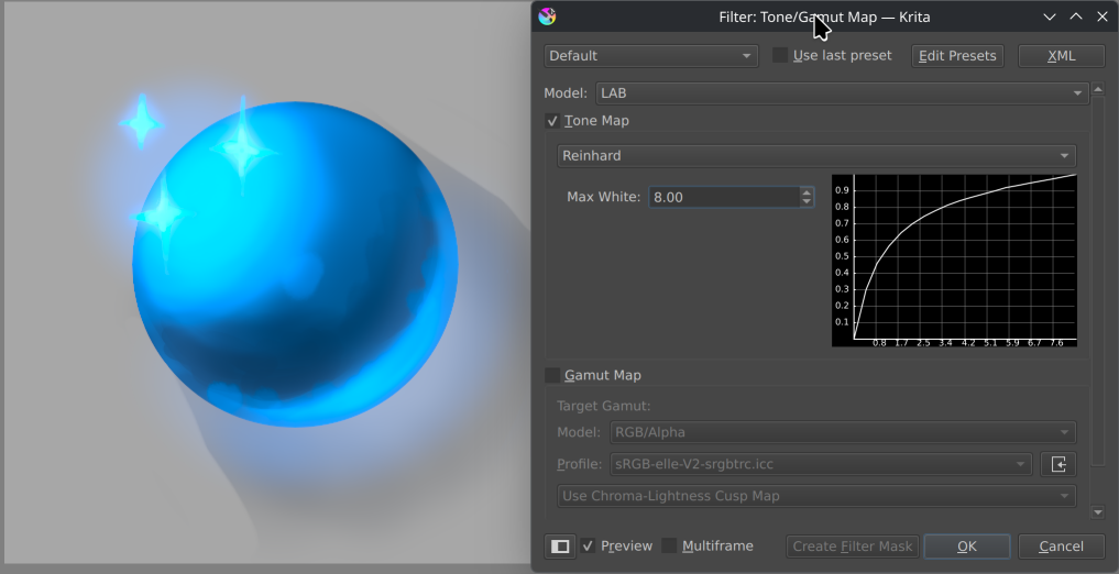
However, we already have a solution to reduce chroma: chroma reduction gamut mapping. So if you apply that after applying the tone mapping, the chromatic highlights get fixed:
Is this better than per-channel tone mapping? I think it depends on the application. Gamut mapping can be quite slow, and isn’t exactly shader friendly, so I can imagine why real-time applications (game engines), would prefer per-channel tone mapping (which more or less does its own form of gamut mapping). Meanwhile, the results of luminance channel tone mapping plus gamut mapping afterwards gives much more chromatic results, which might be more interesting for illustrative works.
Similarly, per-channel mapping only works in a RGB context, and Krita has more models than that to support. By doing our tone mapping in an opponent space, we get the same results regardless of what colour space the image is in, which should make it nice and predictable to work with.
This is one of the reasons that Krita’s tone and gamut mapping filter share the same dialog (they can still be applied separately). The other reason is that we can reduce the amount of colour space conversions if we clump together the two transforms. Furthermore, experience tells me that illustrative artists tend to prefer a single filter here.
OCIO Lut baking
While I was pretty happy with the tone and gamut mapping filter, we were still missing something:
OCIO is the colour management library used by the vfx industry, and it’s strength lies in a big portable configuration that can be much more easily designed that a library of icc profiles. Due this, a well made OCIO configuration often has its own tone mapping solutions, and it would be good if Krita could use these too.
The first thing to decide is what we’re exactly baking. OCIO can be quite flexible, but the way it is implemented in Krita is that we have the standard pipeline provided by OCIO, where we…
- start off in the assigned color space
- go to the config’s preferred linear color space
- Apply the exposure.
- Apply the looks.
- Go to the display color space, apply the view transform.
- Apply the channel swizzle.
- Apply the gamma.
This made things a little tricky, as it is impossible to go from the display colour space back to the assigned image colour space. Furthermore, ideally we’d apply all transforms, including the view transform, so that we get an image that looks exactly like the one you see.
Initially I thought of reducing the scope, and creating a baking transform that applies everything in the config’s preferred linear space, except the view transform. This didn’t work out, as the gamma transform being applied linearly was too unintuitive.
So then, the next attempt was to apply the whole pipeline. This in turn means that the result is in the display color space. This too has some issues, as it requires the display space to be the exact same as the one selected in the preferences. Now, this is required anyway on wayland, as we have no way to determine from a given ocio display what we need to tag the wayland output as. But on the flip side, the default OCIO PQ transform is tied to 100 nits, and we do not yet have the ability to configure the nits level of Krita’s rec2100 PQ surfaces, so the look will remain a little off when using HDR output until we do have that kind of support.
For this reason though, we ask whether you want to convert from the display colour space to the image colour space, or keep the display colour space. That way, the baked result can be quickly saved as an untagged image, like png, and then wrangled by some external script.
Above: Image baked with blender’s current ocio config, using the sRGB display device and the ‘aces 2.0’ view transform.
We’ve had this “Baking” of the config on our wishlist since OCIO was first integrated, so I’m pretty pleased we managed to get it in, even though it still has some papercuts.
Further Work
So, right now, Krita has a built-in tone and gamut mapping filter, which works on luminance, and OCIO lut baking, where the tone mapping generally works per channel. Overall, the OCIO lut baking is probably going to be best for film workflows, while the built-in filter is going to be useful for non-ocio workflows, or when the artist prefers the more chromatic results of the built-in filter.
Because the colourfulness is going to be the key quality of the built-in filter, it’ll be interesting to look at the other gamut mapping options, especially the adjustment-towards-the-cusp.
For CMYK workflows, the gamut mapping filter isn’t too useful right now, as most artists work in sRGB, and the clipping errors towards CMYK there are very rare. Chroma compression might be interesting to experiment with here, but that requires generating a histogram of the chroma over hue, and I’ll need to figure out how to do that while keeping the UI performant.
The built-in filter also doesn’t have adjustment layers enabled just yet. This is because once we allow it as an adjustment layer, we’ll need to always support it. And because there’s a ton of tone-mapping curves out there, and I want to have a period of experimentation before we commit to a particular set.
In the future, I might need to seriously look at splitting up the gamut and tone mapping filters. Benefits here are for example allowing per-channel filter anyway (which is now impossible because the filter tries to find a space that can both gamut and tone map). From further experimentation, I get the feeling that the desaturated results I got tie in strongly with the configuration of the curve, so with a user configurable curve it might get better results. Other things to consider is to allow other models for tone mapping besides LAB and xyY, as that leads to different chromatic colors being applied. At the same time, I don’t want to make this initial filter too complicated.
There’s also some image-aware tone mapping techniques out there. I haven’t investigated them enough though, so I have no idea if they’re useful for Krita’s purposes.
As for which of these is the correct one? That depends on the artist. Tone and gamut mapping are generally considered to be artistic operations, because there’s always trade-offs and only the artist can tell which trade-offs and qualities are acceptable. Hence why I am trying to find a good set of tools for artists to work with.
Appendix
Manually tone mapping.
So, you can sort of manually tone map in Krita, because it supports unbounded workflows. It is a little annoying however, with some pitfalls.
Firstly, you will want to take an HDR image, and scale it’s range into a [0 1] range. You do this by first color picking or using the HDR metadata tab to find the brightest pixel.
Then, you go into the select-a-color dialog by clicking the dual color button at the top. There, you type in the brightest channel value into each channel input. With your HDR color in hand, create a new layer, and fill it with this color. Then set the layer’s blending mode to “divide”. Now the whole image is in a [0 1] range. Then, you can either use the color adjustment filter or the levels filter to make everything visible again, but you will need to use the RGB adjustment, and not the lightness one, as the later goes through lab, and somehow that means everything gets desaturated.
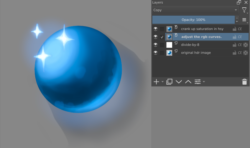
This generally desaturates the whole image a little, as it is a form of per-channel tone mapping, so I personally pump up the saturation after my levels corrections.
The other pitfall here is that it becomes really hard to get a good curve the higher the brightest white is, because the curve needs to be fine-tuned more and more to both get nice shadows and nice highlights at the same time. The tone mapping filter is easier to use, in this case.